CPSC 330 Lecture 3: ML fundamentals
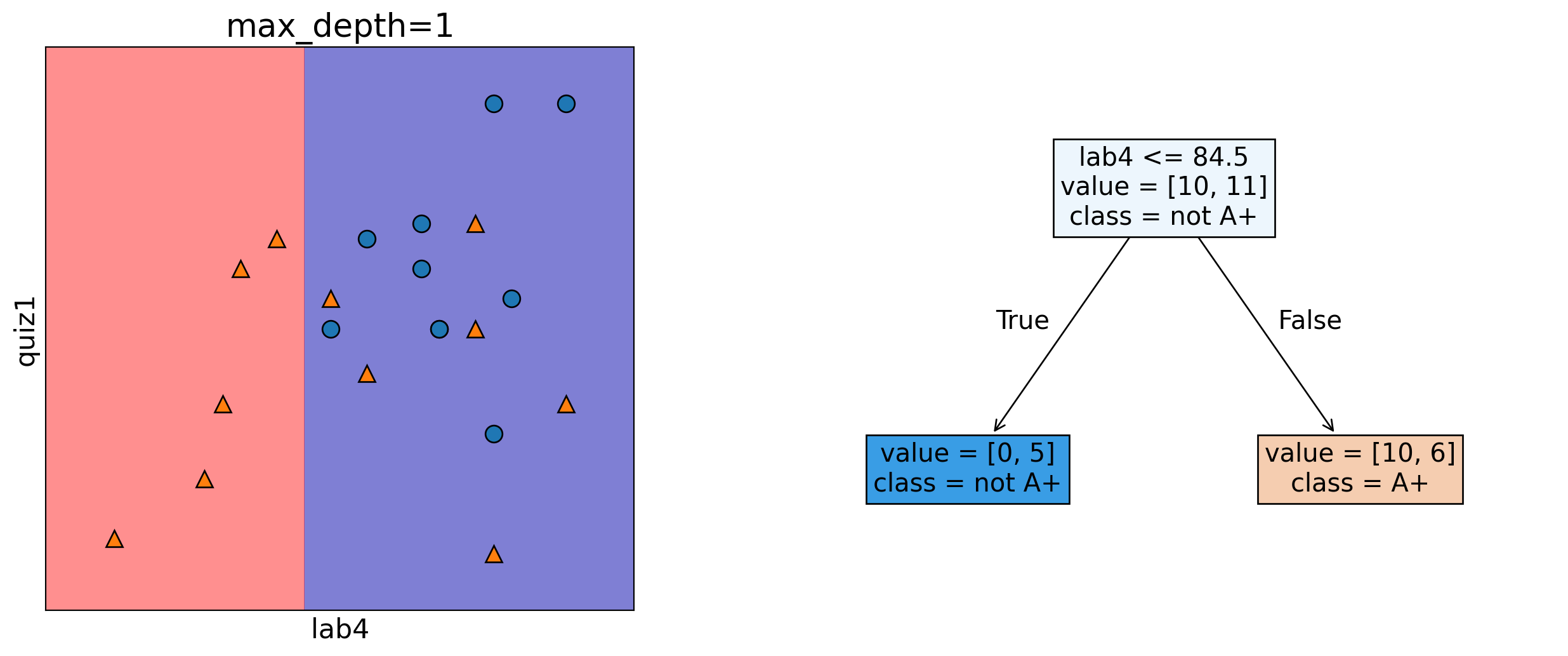
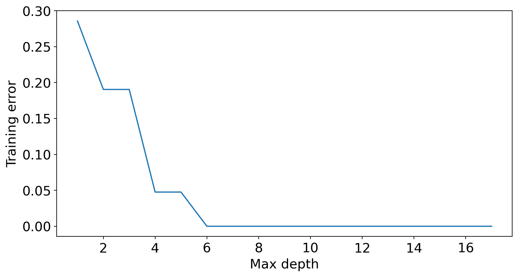
Depth = 1
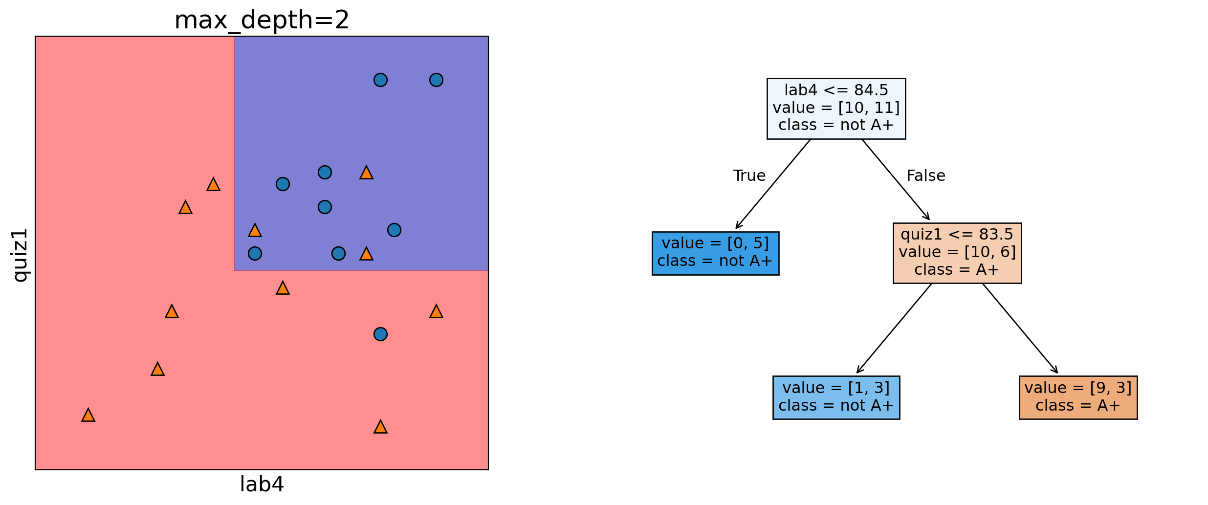
Depth = 2
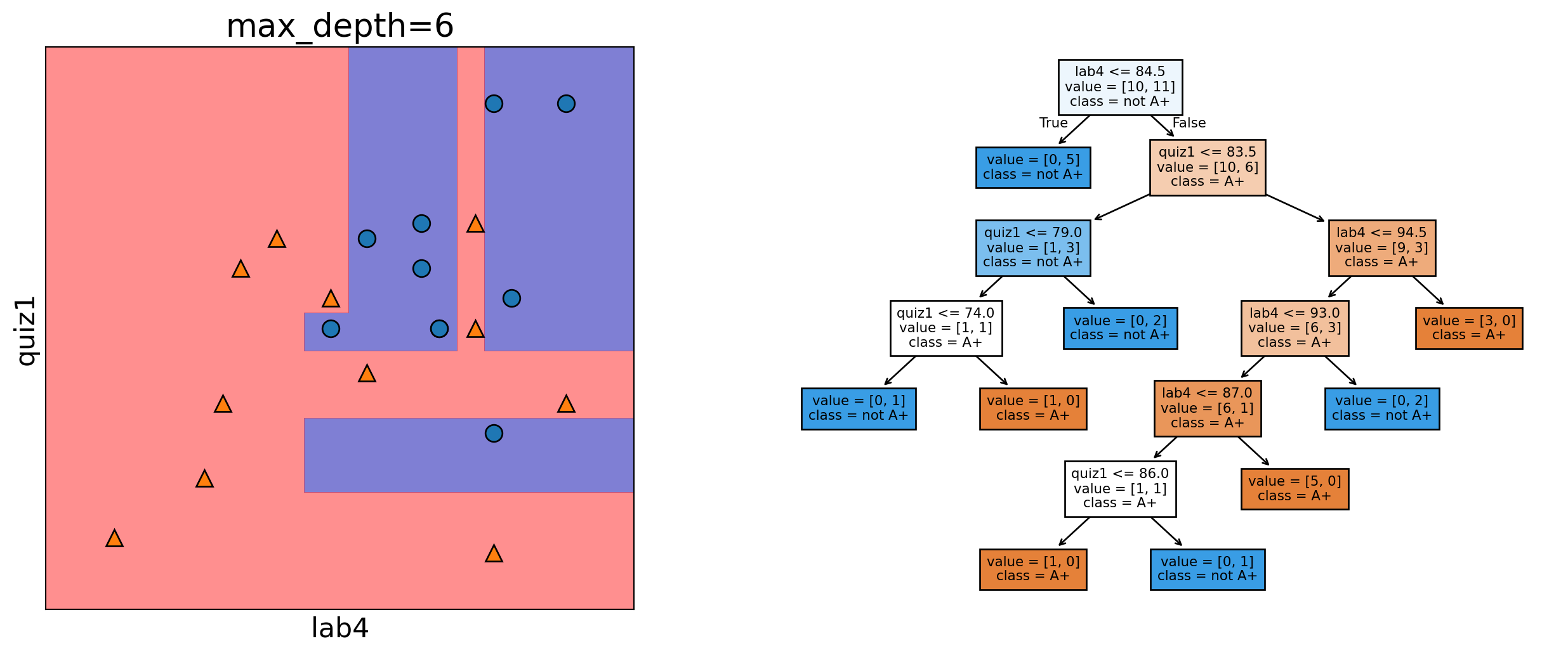
Depth = 6
Complex models decrease training error
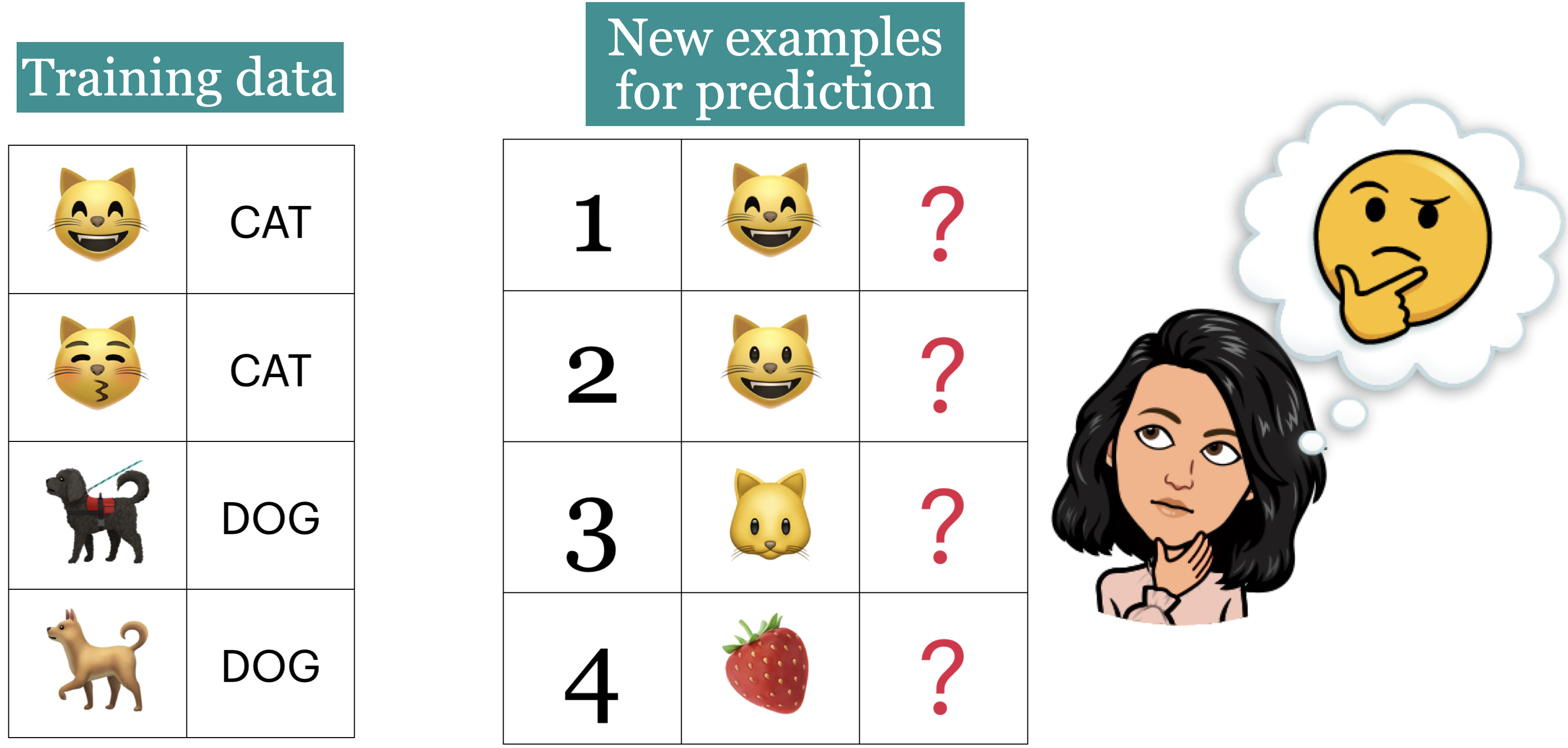
Generalizing to unseen data
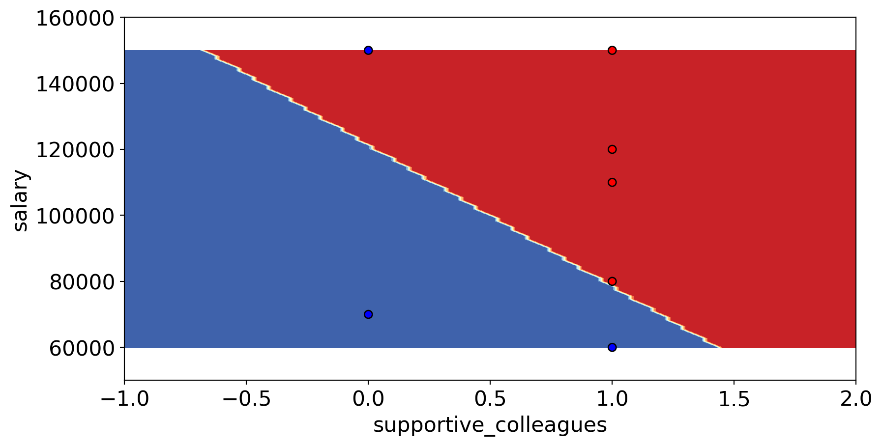
- What prediction would you expect for each image?
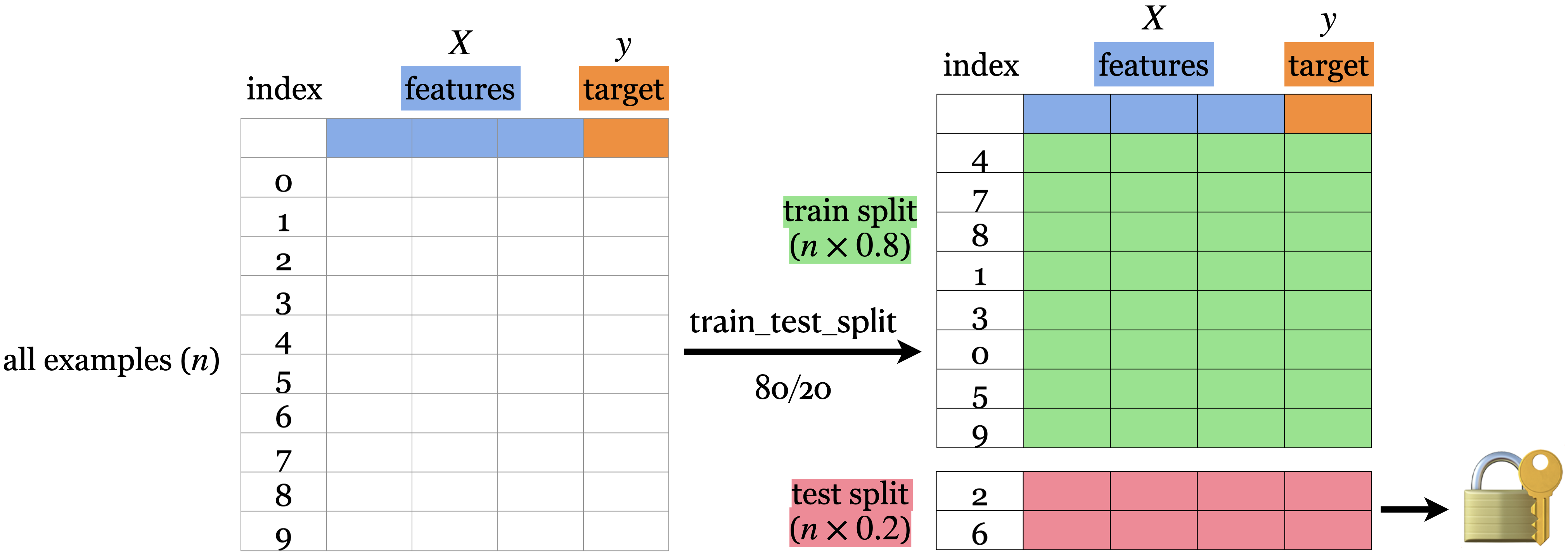
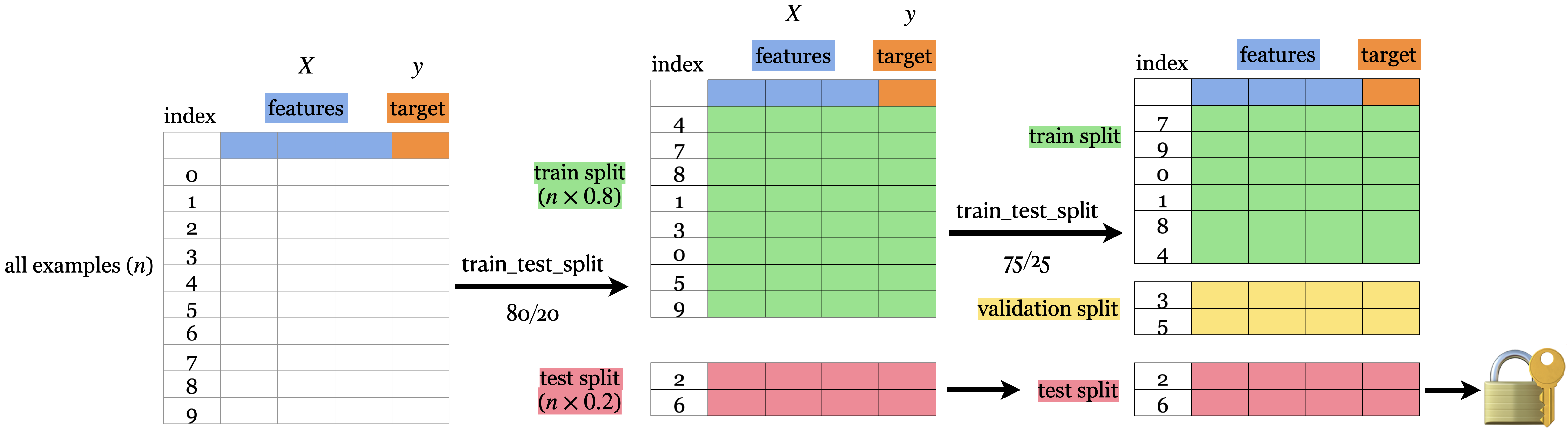
Train/test split
Training vs test error (max_depth=2)
Train error:   0.125
Test error:   0.400
Training vs test error (max_depth=6)
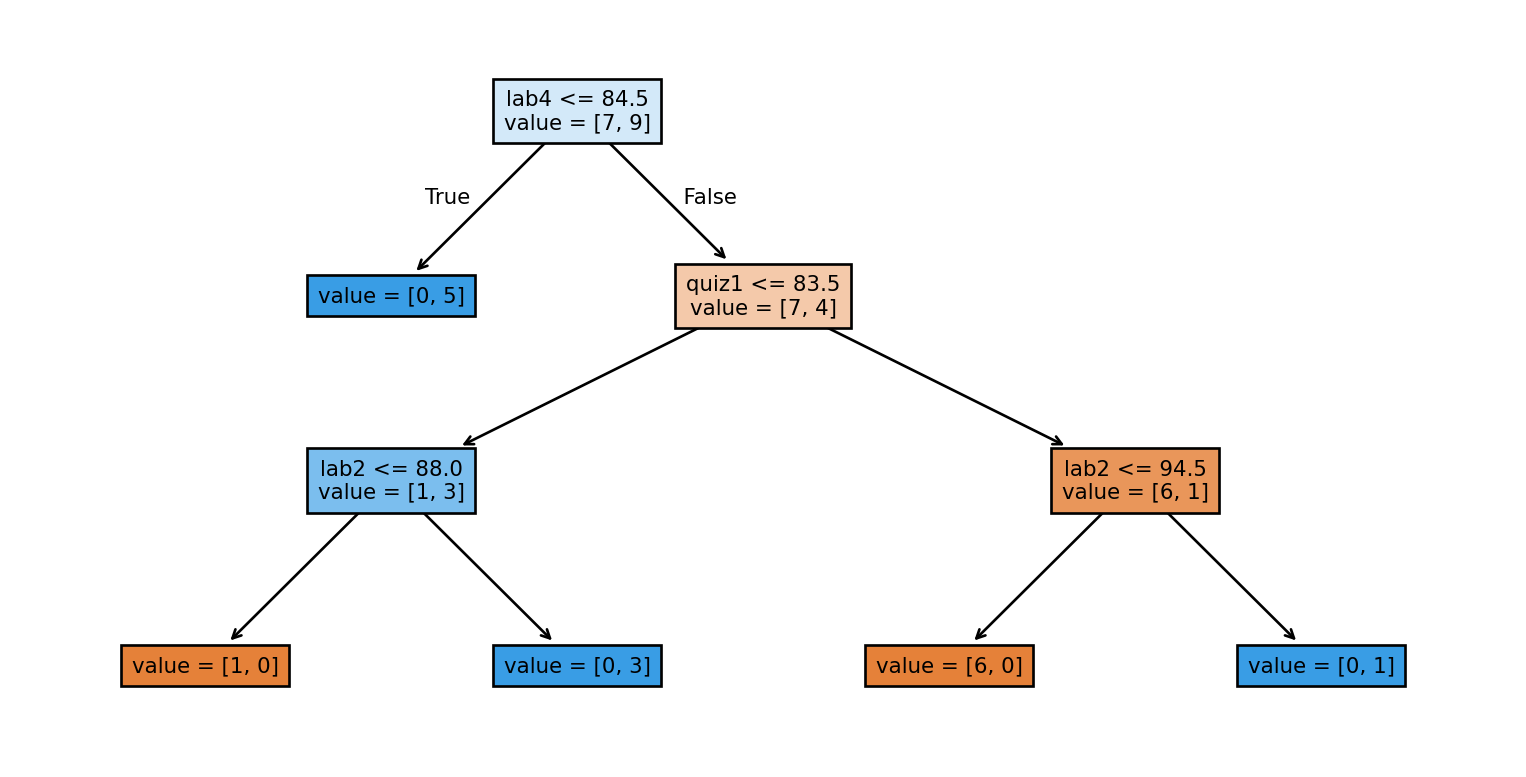
Train error:   0.000
Test error:   0.600
Train/validation/test split
- Sometimes it’s a good idea to have a separate data for hyperparameter tuning.
Problems with single train/validation split
- If your dataset is small you might end up with a tiny training and/or validation set.
- You might be unlucky with your splits such that they don’t align well or don’t well represent your test data.
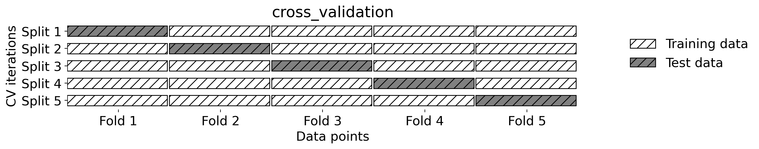
Cross-validation to the rescue!!
- Split the data into \(k\) folds (\(k>2\), often \(k=10\)). In the picture below \(k=4\).
- Each “fold” gets a turn at being the validation set.
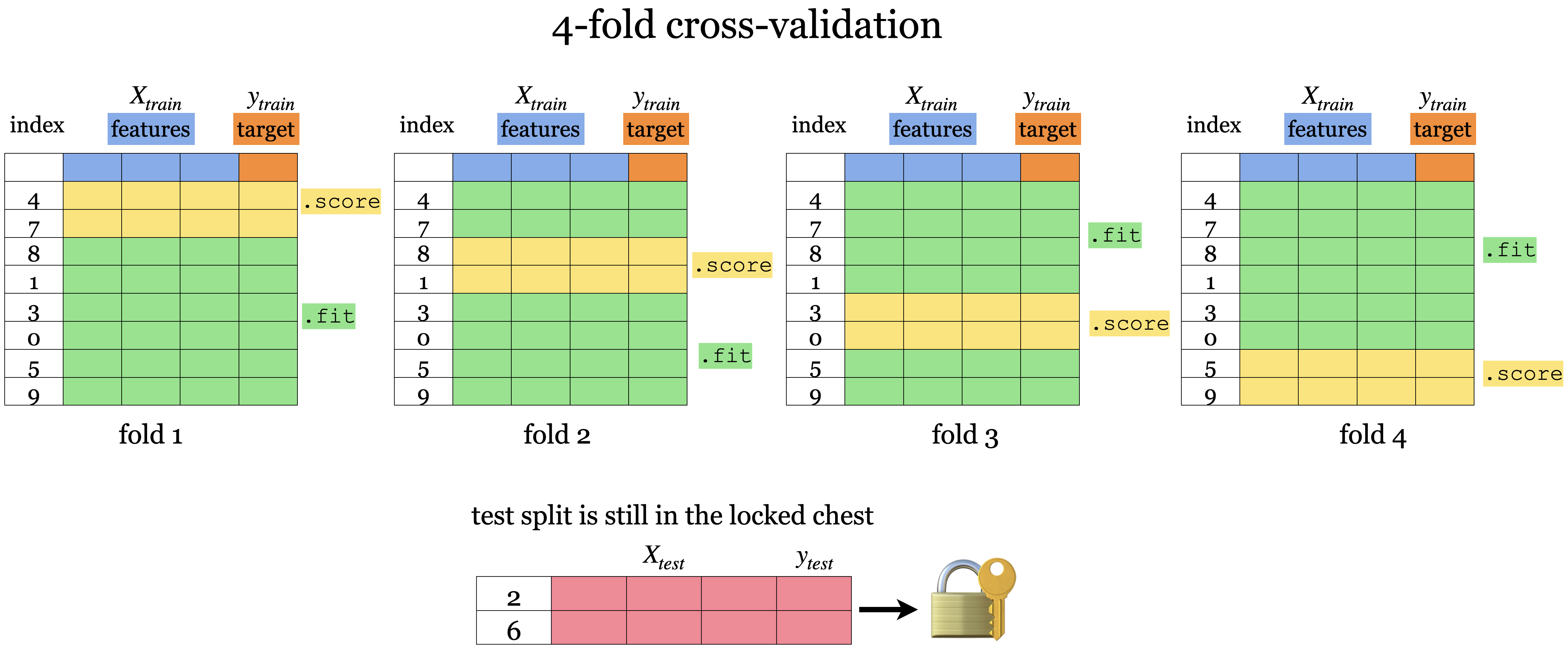
Under the hood
- Cross-validation doesn’t shuffle the data; it’s done in
train_test_split.
How to pick a model that would generalize better?
- We want to avoid both underfitting and overfitting.
- We want to be consistent with the training data but we don’t to rely too much on it.
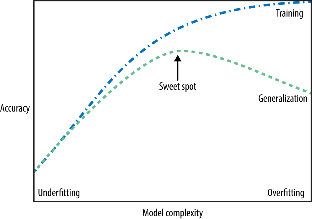
There are many subtleties here and there is no perfect answer but a common practice is to pick the model with minimum cross-validation error.
Class demo (Time permitting)
Copy this notebook to your working directory and follow along.
![]()